The Production Possibilities Curve

The Production Possibilities Curve is a tool used to illustrate the concepts of scarcity and choice in an economy. It is not an economic law or an illustration of a real economy. Instead it is a simplified illustration showing a hypothetical economy that produces only two products. The curve shows that, when using all of its resources, the only way to increase the production of one product is to reduce the production of the other. Limited resources mean we have to make choices and the Production Possibilities Curve demonstrates this graphically.

Let's assume that some alumni of the college dies and, in his will leaves a small building in a strip mall to the college. The mall and building are about five miles from the campus. Instead of selling or renting the building (which is what colleges usually do with gifts like this) the college decides to use the building for desperately needed classroom space. Leaving the small reception area in the front of the building, they remodel the building into two classrooms – a 30 seat regular classroom and an 20 seat computer lab. They then hire an instructor, who can teach both economics and computer science, to teach eight classes per day at this satellite site. Since the instructor can only teach one class at a time she alternates between computer and economics classes. The maximum number of classes that can be taught per day is eight and the only way to increase the number of computer classes taught is to reduce the number of economics classes and vice versa.




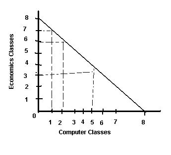
In the above example the production possibilities curve was a straight line indicating that a constant opportunity cost whereby the opportunity cost of one additional economics class is one computer class and vice versa. However, in real life the trade-off or opportunity cost is usually not constant for the entire length of the curve. This is because when we are in the middle of the curve and producing both products we usually can switch resources from one to the other and increase the output of good 'A' by one by decreasing the output of good 'B' by one. However, as we approach either end of the curve and seek a further increase in good 'A' we find that we have to give up increasing amounts of good 'B' in exchange. This is known as the Law of Increasing Opportunity Costs and is depicted by a production possibilities curve that is bowed outward rather than as a straight line as in our first example.

The reason for increasing opportunity costs is the fact that all resources are not variable. Let's modify our example by adding a second instructor who only works in the mornings. Like the first teacher, he can also teach either economics or computer science. In the morning we can now have four economics and four computer science classes and in the afternoon we can have four additional classes of economics and computer science. However, the total number of classes we can teach per day is 12 and the maximum number of either class we can teach using that class's designated room is 8 (in the morning we can teach 4 of each class and in the afternoon we can do up to four of one or the other). Since the economics classroom holds 30 students and the computer classroom holds 20 we can teach up to 240 economics students (30 students times 8 classes) or up to 160 computer science students (20 students times 8 classes). The opportunity cost of teaching an additional 30 economics students per day is 20 computer science students and vice versa. But, what if we are offering eight economics classes and four computer classes and wish to add one more economics class? Both teachers can teach either course so our labor is perfectly flexible between the two subjects. However, to add a ninth economics class means that both teachers will have to teach economics at the same hour in the morning and this means that one teacher will have to teach economics in the computer lab which only holds 20 students. Because our land (rooms) resource does not adapt as easily, it still costs us a loss of a class of 20 computer science students to be able to teach the additional economics class but, due to the room configuration we can only teach 20 (rather than 30) economics students. Similarly, since there is only one computer in the economics classroom we would have to reduce the number of computer science students taught if we added a ninth computer science class by using an economics room to teach computer science (in order to give each student sufficient time on the computer we would probably have to limit the class to 7 or 8 students).




Points inside or outside the curve. In the second graph above point 'B' is inside the curve and point 'C' is outside the curve. Point 'B' represents unemployed resources. This is inefficient because society is not using all of its available resources and, consequently, is not producing as much as it could. If society is a point 'B' it means that it could increase output of both to produce MORE of each good. In our example let's assume that on the main campus, to avoid congestion in the halls between classes, they start computer classes on the half hour and other classes on the hour. Both types of classes are an hour in duration but they start and end at different times. Assume that the scheduler makes a mistake and applies this rule to the classes at our satellite. Now, instead of moving from one class to another our first professor has a half hour wait whenever she switches from an economics class to a computer class or vice versa. There is no way this professor can work from 8 – 5 with an hour off for lunch and teach eight full classes of economics AND computers with the schedule configured this way. She will face at least one or, depending upon the combination of classes, more half hour periods of "unemployment". If our professor is being paid by the class she will suffer a loss of income and, with class offerings reduced, fewer students will be able to take the classes each semester. Even if our professor is paid the same salary as before the financial cost of her "unemployment" will just be shifted to the students as the college will be forced to increase tuition to cover the loss of revenue from the canceled classes. Or, if this is a public college and we don't increase tuition we will have to obtain the lost revenue from the taxpayers – there is NO FREE LUNCH as someone or some group always has to pay.

The other point on the second graph, point 'C' represents a combination of classes that is not possible with existing resources. This is more than we can produce at this time. However, this does not mean that we can NEVER reach this point. Economic growth (an expansion of the economy's output capability) will cause the Production Possibilities curve to shift outward. An increase in labor could give the economy the boost it needs to increase output. This can be in the form of having more children (but this process takes twenty years or more as we have to wait until the children grow up an acquire skills); immigration from abroad; or, new technology that allows society to better utilize existing labor (the invention of the typewriter enabled people with poor handwriting skills – i.e., you could not read their handwriting – to produce readable documents. An increase in land could result in economic growth. This could take the form of draining swamps, irrigating deserts, adding artificial fertilizer to existing land, terracing the sides of mountains, etc. An increase in capital could also result in economic growth. This could come from the savings of society as society reduces consumption and diverts the saved resources to the production of capital goods. It could also come from investment in capital by foreigners seeking to increase their profits by building new production facilities in our country. Finally, new technological advances that result in existing land, labor or capital becoming more efficient will also result in economic growth.