Why Do the Prices of a Bond Fluctuate between Issue and Maturity?

A student recently asked why the prices of previously issued bonds fluctuate even though they have a face value of $1,000 which the current owner receives when the bond matures.

Bonds are debt insturments issued by corporations and government entities. Basically, the business or government (the Federal, state, local or an agency like FNMA or entity like Pima College) has a need for a large sum of money and raises that sum by selling bonds. Bonds are usually issued in $1,000 units – that is, each individual bond has a value of $1,000. Most bonds have a fixed interest rate and are usually redeemable in 25 - 30 years (i.e., the buyer does not get their $1,000 back for 25 - 30 years). Interest is paid quarterly, semi-annually or annually for the life of the bond by the issuing authority and the principal (the $1,000 the buyer paid for the bond) is re-paid at maturity (25 - 30 years later). The interest rate is fixed and that is the rate the issuer pays to the owner of the bond during the life of the bond.

If the buyer of the bond wants her money back before the bond matures in 30 years she can sell it to another person. For instance, I may buy a bond paying 10% interest with a 30 year maturity. Five years later I need money to help pay my child's college tuition. So I sell the bond to you. While I owned the bond I received the interest payments. Now that you own it they are sent to you. If you hold the bond to maturity you will receive the $1,000 face value (i.e., what it was originally sold for) that I originally paid. But you can also sell it to someone else if you do not want to wait until maturity for your money.

While the face value of the bond does not change, the amount subsequent buyers are willing to pay does change. Interest rates are the main thing that causes bond prices to change when they are traded before maturity (there are some other factors influencing the price as well but we can ignore them for now). Assume that rates were 5% when I brought the bond and that is the rate the bond pays. Pima College or IBM or whoever issued the bond is obligated to pay $50 per year (05 * 1,000) to the owner of the bond. Now suppose five years have gone by and I want to sell this bond paying 5%, but interest rates are now 10%. You are not going to pay me $1,000 for this bond paying $50 per year when you can buy a new bond being issued by some other company or government paying the current rate of 10% or $100 per year. To get you to buy my 5% bond I have to lower the price to the point where the $50 per year being paid is equal to 10% of what you paid me for it. Therefore, I will sell it to you for $500 so that the $50 annual interest paid on the bond is equal to 10% of the amount you paid for the bond.

Similarly if I had purchased a bond that paid 10% interest and rates dropped to 5% then numerous people would want to buy it from me for $1,000 so they could get 10% rather than the current 5% on their $1,000 investment. These people would compete for the bond and bid its price up until it reached $2,000 (at which point the $100 per year interest being paid would be a 5% return on their $2,000 investment).

This is why bond prices fluctuate as interest rates fluctuate when they are resold or traded before maturity.

Tax Cut Article - Part 5 of 5

We now come to the last part of the question and that refers to the quality of the jobs being created.

Like the Reagan tax cut in the 1980s, opponents of the Bush tax cut are reluctantly conceding that the tax cut is creating jobs, but they criticize it for both not creating enough jobs and for creating mostly lower wage jobs.

The simple response to this is that, since there are more entry level and other lower end jobs than there are higher end jobs, it is logical that there would be more lower end jobs created. Remember the story about Ronald Reagan when he was an actor and limited himself to making five movies per year because the high marginal tax rates would tax away most of the earnings from the sixth. It was pointed out that, in addition to Reagan voluntarily making himself unavailable for a sixth movie, all of the lower paid supporting cast as well as support crews also lost out on the chance to be employed on the sixth movie.

New jobs are being created at both ends of the spectrum and in the middle but, since higher end positions usually require many more lower paid positions to support them, more lower end jobs will be created. Also, many of the new higher end jobs are taken by people who are already employed and see a chance to move up or people, like Ronald Reagan, who are not unemployed, in the sense that they have voluntarily limited the amount of work they do, and are now incrasing their employment activities in response to the new tax environment.

Another factor, usually not considered by the media and oposition politicians, is the fact that, due to increasing efficiency and output per worker, money wages are flat or increasing slowly while prices are falling. The falling prices mean that real wages (the amount that the money wages will buy) are increasing. This means that, despite the fact that money wages are not rising, workers are able to afford more with the money wages. This is the same as a raise in money wages when prices are constant. This is called secular deflation and occurs when the aggregate damand curve remains relatively constant while the Long Run Aggregate Supply Curve keeps shifting to the right as output keeps increasing.

The job quality issue, like the other aspects of the tax cut, can be looked at in more than one way depending upon the viewer's perspective. What is happening is that our economy is moving away from central management from Washington and toward a more free market model. The majority of the people benefit from this in the form of more products and lower prices and this is good. But there are some losers and they are the ones who were fortunate enough to get jobs in protected areas (such as unionized manufacturing) where the government protected their high wages from competition. But the cost of that system of protecting the higher than average wages of certain groups of workers came in the form of everyone having to pay higher prices.

Tax Cut Article - Part 4 of 5

Has the Bush Tax Cut Created Jobs?

Today we will deal with the next part of the question which is how effective has the tax cut been in creating jobs?

As I indicated in yesterday's article, there is a lag between the time the tax cut is enacted and the time households respond to the new environment. Since the tax cut was across the board in that it affected all income brackets, there was some Keynesian style stimulus on the demand side as many of the recipients began spending this money. As people began spending the additional money from the tax cut there was an increase in demand and business responded by drawing down inventories and hiring more people to increase output to replenish the inventories.

The most recent figures from the Bureau of Labor Statistics' payroll survey show an increase of 2.4 million jobs from August 2003 through October 2004. The Department of Commerce's household survey shows an increase of 2.5 million jobs for the same period. The difference is that the BLS figures are based upon a survey sent to existing businesses while the Commerce figures are based upon a survey of households which include people who have started their own business or work for very small new businesses both of which are overlooked in the BLS survey.

In addition to the 2.4 or 2.5 million new jobs created, the national unemployment figure for October 2004 was 5.5% which is down from the peak rate of 6.3% in June 2003. It is also lower than the average rate in the 1970s, 1980s and 1990s. Another encouraging sign in the 5.5% rate for October was that it increased by a fraction of a percent over the September figure. This is encouraging in the sense that one sign of an improving employment picture is an increase in the rate of unemployment. If you review the discussion of unemployment in your text you will notice that the official definition of unemployment is people who are both out of work and actively looking for work. If laid off workers get discouraged and stop looking for work, as happens in recessions, they are no longer included in the official unemployment statistics. When the job market improves, as it is doing now, these people begin looking for work again and they are reclassified as unemployed and are again included in the unemployment statistics.

So, with all this good news why do we hear so much about the tax cut not working? Obviously, during the recent election Senator Kerry and the other Democrats opposing President Bush and the Republicans could not praise the President for his good job and, at the same time, try to convince people to vote him out. Much of the mainstream media and others oppose President Bush and the policies that he is pursuing so they will naturally be critical of his policies. This is normal political debate.

But there are also some legitimate grounds for criticizing the effectiveness of the tax cut and of President Bush's economic policies in general. Like any policy, President Bush's economic policies in general and the tax cut in particular, are not perfect. If they were we would have zero unemloyment, stable prices and overall prosparity. Obviously this would be impossible to achieve, but to the extent we fall short of this ideal there is room for opponents to criticize the Presient's performance and put forth alternative policies that they feel will do better. In the recent election the voters could see the results to date of the President's policies and had to estimate how accurate the claims of the effectiveness of his opponents' proposed policies were. To the extent that people based their votes on economic considerations, we can say that a majority of the electorate felt more confident in staying with the existing policy than taking a chance on the alternative policies.

A second reason for questioning the effectiveness of the President's policies is the fact that the U.S. Is a large and diverse nation and the increase in jobs is not evenly distriubted throughout the nation. The Administration's own web page contains data that can be read in either a positive or negative light. According to the Administration, Job creation was up in 47 of the 50 states in the last year, and the unemployment rate was down in all regions and in 46 of the 50 states. This is good news if you are employed and living in one of the 47 states where job creation was up or one of the 46 states where unemployment was down. But what about unemployed people in the three or four states where jobs were not being created rapidly or unemployment was not going down? They obviously have a different perspective.

So, short of the policy either working spectaularly or failing massively, the relative effectiveness of the policy will depend upon each individual's point of view and opinion of the current and alternative policies. My job as your instructor is to teach you the principles of economics and provide you with a clear understanding of the various theories behind the competing policy positions. The decision as to whether a particular policy is better or more effective than competing policies is up to you but, hopefully, as a result of this class your opinion will be backed up with an understanding of the principles and theories involved and not rely upon political hype alone.

Tax Cut Article - Part 3 of 5

Where the Bush Tax Cuts Effective?

Part of the student's original question was "...would you say President Bush's tax cuts were ineffective because of the deficits they created?"

The idea behind the supply side type tax cut that President Bush signed into law is that marginal tax rates are too high and these high rates discourage discourage people from increasing their incomes by working more. The idea is to reduce the rates to encourage more work which means more income is earned and that increases the amount of income available to tax. In theory the increase in income due to the tax cut will be proportionately larger than the percentage reduction in tax rates so the new, smaller tax rates times the new higher incomes will produce more tax revenue. As an example, ten percent of $100 is $10 while 8% of $150 is $12. In this example the smaller rate against the larger base resulted in a larger amount collected ($12 rather than $10).

There is a lag between the passage of the tax cut and the time the people adjust their work hours. Once a tax cut law is passed people see that they can keep more of the extra money that they earn and are then more receptive to additional work. But actually increasing work hours takes time. When companies have the need for overtime work they will find employees more willing to volunteer for such work. Also, some people will begin looking for part-time jobs to supplement their incomes, stay at home spouses will find it advantageous to return to work, and high income professionals will find it profitable to increase their service offerings.

Ronald Reagan used to tell the story about when he was a movie actor he found that he could live very well doing five movies per year. But if he did a sixth movie it pushed him into a higher tax bracket and most of the additional income from the sixth movie went to taxes. So he limited himself to five movies per year. It was not just Reagan's income from the unmade sixth movie that was lost to the IRS but also the incomes of all the other minor actors and support people – people whose incomes were much less than that of the star, Reagan, and who wern't faced with losing most of the extra income to the IRS but they, and the IRS, lost out on that extra income because the sixth movie was not made. Multiply this by all the high paid actors, lawyers, doctors, etc. who deliberately limit both their hours and the hours of their staffs and you can see that large amounts of income are not being made and thus, not available to be taxed.

Initially taxes are cut and the tax base, or total income being generated by taxpayers, remains the same so tax revenue falls. To avoid a deficit, the government should make a corresponding reduction in spending but this never happens. Remember, this was the reason the Republicans originally opposed the Kennedy Johnson tax cut was fear of the deficit. But, once the tax cuts take effect and people have time to adjust, incomes increase and this results in a larger tax base which generates the revenue to remove the deficit.

That is the theory. There is a caveat and that is that the politicians cannot be allowed to increase spending to match the increase in revenues. Government's are like my children, they can't resist the urge to spend all the money at their disposal. In the case of my children the cost of lunch in school is three dollars, but if I only have five dollar bills when I drop them off at school they manage to spend the entire five rather than bringing home the change.

The Kennedy Johnson tax cut increased revenues but, in addition to the tax cut which caused a short term deficit, President Johnson also enacted the very expensive Great Society program AND attempted at the same time to finance both the Vietnam War and the Cold War. This was too much and massive inflation followed.

Ronald Reagan's tax cut resulted in a short term deficit but he fought hard to keep spending in line and was aided by this with the Gramm-Rudman-Hollings law which required Congress to find money to pay for new programs before they could enact the programs. The result of the Reagan tax cut was over a decade of economic growth, low inflation and a budget surplus (which has since been spent by his successors).

There is reason for concern about the deficit with President Bush. Unlike Reagan, whoes philosophy was "The government is the problem" and sought to reduce government spending, President Bush's compasionate conservatism tends to see government spending as a problem only to the extent that it is not being managed responsibly. President Bush does not seem to be philosophically opposed to big government and big government spending per se.

The tax cuts are starting to increase revenue as expected. But there is anger and concern among many of the President's supporters because of his tendency to approve big spending items like the Medicare Prescription Drug law, the No Child Left Behind Act, etc. all of which represent huge increases in spending. Some of his supporters give him the benefit of the doubt by saying that he included free market incentives in the laws such as the Health Savings Accounts in the Medicare bill and the accountability rules in the NCLFB act and that the increases in spending were required to get these needed structural reforms passed. We will have to wait to see how he handles spending in his second administration before we can conclude whether the initial deficit from the tax will be a problem or not. But regardless, the tax cut is generating economic growth and the revenue to eliminate the initial deficit. The only question is will the administration and Congress use the money to eliminate the deficit or go on a spending spree.

Tax Cuts and the Economy - Part 1 of 5

The following question was received from one of the students in the Economics 200 course:

From an economist's perspective, would you say President Bush's tax cuts were ineffective because of the huge deficit they created? Also they haven't seemed to stimulate the economy that much or create many more high jobs and the cuts were done during a war?

Here is my reply to this student:

This is a very good question. However, your question has three parts and I will answer each in a separate article. The three parts of your question are:

1. The budget deficits that resulted from the tax cut

2. The amount of jobs created as a result of the tax cut.

3. The quality of the jobs created.


The first thing to keep in mind is that tax cuts are as much political as economic, meaning that the President and Congress are just as concerned, if not more concerned, about the political as the economic effects of a tax cut. There are two main economic theories behind tax cuts: the Keynesian theory and the Supply Side theory. There are also two main political motivations behind tax cuts: increase government control of the economy or reduce government control of the economy. The economic theories are not necessarily mutually exclusive as was demonstrated when President Bush and some of his supporters used both Keynesian theory and Supply Side theory arguments when arguing in favor of the tax cut plan. The political motivations, however, are mutually exclusive in that the motivation must be for either increasing or decreasing the size of the government as you cannot do both at once. It is the political motivations behind tax cuts that divide Republicans and Democrats.

Let's start with the economic rationale for tax cuts and look at the two theories behind them.

The first theory is the Keynesian theory which views tax cuts as a counter cyclical tool of fiscal policy. Keynes focused his theory on demand and viewed demand as the key to managing the economy. Writing during the Great Depression of the 1930s, the problem Keynes saw was an economy faced with massive unemployment of both labor and the other factors of production. The problem, as Keynes saw it, was inadequate demand – people were out of work and and their purchasing power was sevearley restricted. With sales slow to non-existant, employers could not afford to hire people if there was no one to purchase their product. Classical theory stated that, in a free market, prices would fall to the point where people could afford to purchase the goods and wages would also fall to where employers could afford to begin employing people again. As the economy expanded wages would begin to rise as employers were increasingly forced to lure additional workers with the promise of higher wages. But the 1930s were not an era of flexible wages and prices. The economy was heavily unionized and union contracts would not allow wages to fall. Similarly, cartels existed in many industries and these acted to limit output and maintain price floors. Since normal free market mechanisms were not working, due mainly to unions and cartels, Keynes felt that the only way to pull the economy out of the depression was for the government to move in and act as the catalyst to get the economy going again (actually, it was government policy that provided the unions and industrial cartels with the power to enforce the wage and price floors). According to Keynesian theory, when the economy was in a recession or depression the government was supposed to step in and increase demand by:

1 increasing government spending (on things like building roads, public buildings, etc.) while not increasing taxes;

2 by cutting taxes while maintaining current spending levels; or,

3 a combination of increasing spending and cutting taxes.

Any one of these three courses of action would mean that the government was spending more than it collected in taxes and this would result in a budget deficit. But deficits were the goal of this policy as the objective was to keep government spending level or increasing while also increasing consumer spending.

Supply side theory stresses the need to increase supply by growing the economy. Modern supply side theory came into vogue during the 1970s and 1980s when the economy was expanding and demand was exceeding the economy's capability to produce goods and services to meet the demand. The problem was inflation, not depression. According to the theory, tax cuts were needed not so much to stimulate demand as to grow the economy. It was felt that tax rates were such that they were discouraging investment and work. Economist Arthur Laffer developed a curve showing that as marginal tax rates (see the October 10th posting on the Progressive Income Tax) increased they reached a point where they discouraged additional work and investment. By reducing the high marginal income tax rates government would let people keep more of the additional money that they earned – i.e., overtime income, income from a second job or income from a spouse going to work. People have to put forth a certain amount of work in order to support themselves, but, they will only work additional hours (overtime, second job, spouse going to work) if they see some reward in it. If the government taxes away most of the additional income people will have no incentive to put forth the extra effort. When existing workers work longer hours it is the same, in terms of production, as increasing the number of workers. For example, if ten people accept overtime assignments of four hours per week each (i.e., each worker works their regular 40 hours per week plus 4 hours of overtime) this is the same as adding one additional worker to the labor force. If one million people work an additional four hours per week that is the equivalent of adding 100,000 workers to the labor force – you can see that this could increase output substantially.

Note that after point 'X' on the graph, additional tax increases result in REDUCED revenues. If you are in the area to the right of point 'X' then REDUCTIONS in tax RATES will result in more revenue. But if you are to the left of point 'X' then reductions in rates will result in reduced revenues for the government.

In the next posting I will discuss the politics behind tax cuts.

Arbitrage

A take home test question in one of my four classes concerns the term arbitrage. In the text for the course the term is defined as "buying low and selling high".

Essentially arbitrage involves buying an item at a low price in one market and selling it at a higher price in another market. One of the roles of an entrepreneur is to identify items that are relatively scarce in one market (and hence have a high price) but are abundant in another market (as reflected by a lower price in that market). The arbitrageur then buys the product in the market with the low price and re-sells it in the market with the higher price. Obviously, this will increase the demand for the product in the lower priced market causing the demand curve to shift to the right and the price to rise. In the higher priced market the increased supply of the product that results from the entrepreneur or arbitrageur's action will cause the supply curve in that market to shift to the right causing the price in that market to fall. Eventually the two prices will converge and the price will be the same in both markets.

For arbitrage to take place there must not be any insurmountable barriers to the transaction. For instance, fresh lobsters are cheaper in the coastal areas of Maine than in Arizona. Restaurant owners in coastal Maine simply go to the dock and buy the lobsters from the returning fishermen. In Arizona the lobsters have to be packed and flown across the country causing the price to be considerably higher. But an arbitrage opportunity does not exist because the price difference is due to the shipping costs which cannot be avoided.

Generally, arbitrage opportunities arise due to lack of easy access to information and markets. But once these are overcome opportunities for arbitrage appear.

A decade ago the market for antiques and collectables was fragmented and localized. Potential sellers tended to be individuals with limited information about the market and too few items to justify the time and expense to seek out buyers for their items. Buyers also tended to be small collectors with limited resources. Enter eBay. With a few keystrokes and payment of a very nominal fee, sellers could advertise their wares to the world. With the same few keystrokes and no monetary cost, buyers could literally search the world for the items they desired. Prices were determined by demand and supply in this world wide market and everyone had immediate access to the latest price information in the market. Thousands of people found that items cluttering their homes were fetching high prices in other parts of the country and, for a nominal fee to eBay and a small shipping expense, they could reap a large profit on these previously "worthless" items. The result was an explosion in antiques and collectables with people first selling the accumulated clutter in their own homes and then, the more enterprising ones, branched out and began shopping garage sales, estate sales, local antique shops and auctions seeking items that could be sold for higher prices in other areas. It didn't take long for everyone to learn about eBay and the opportunities for profit. Today, most arbitrage opportunities in this market are gone as the market done its job of transmitting information and eliminating price differences between different areas for the same items.

Supply and Demand Explained

Demand Curve – shows quantities of a good demanded (that will be sold) at various prices. The higher the price the lower the quantity demanded and vice versa.

Think of it this way, if you have $10 in your pocket and an item costs $10 you can afford to purchase one unit of the item. But if the price is $5 you can afford to buy 2, and if price is $2.50 you can purchase 4, etc.

Further, since there are more middle and lower income people than rich people, the lower the price the greater the number of people who will be able to afford to buy the product and the more people able to afford the product the greater the quantity that will be demanded.

Supply Curve – shows quantities of a good supplied at various prices. The higher the price the greater the quantity supplied.

No business (supplier of a product or service) can afford to sell at a price lower than cost and remain in business. BUT all suppliers of a good do not face the same set of costs. A farmer with fertile soil, a good climate and sufficient rain can produce a larger crop, at a lower cost than a farmer growing the same crop in poor soil in the desert. The desert farmer incurs the same costs for seed, labor, etc. as the other farmer. But the desert farmer must also purchase fertilizer, install irrigation and pay for water. As a result, the desert farmer will have higher costs per bushel of product than the farmer in the ideal location. In order to make a profit on his crop, the desert farmer has to receive a higher price per bushel than the other farmer. The point is that producers of a good or service face different circumstances and some are able to produce at a lower cost (require fewer resources) than others. As the price of a good rises more producers are able to offer the good or service.

As a second example, consider yourself and the sale of your labor services. If you had tickets to a concert for tonight and your supervisor asked for a volunteer to work overtime at the regular hourly rate you probably would not volunteer. If double time was offered, you might be tempted but the desire to see the concert would probably be greater. But, if your supervisor offered a $1,000 bonus to put in an additional four hours this evening, doing your regular work, you would probably take the offer. As the price goes up you, as the seller of your labor services, are more inclined to increase the quantity of labor you are willing to provide. In this example the cost is your opportunity cost. If you earn $10 per hour and your concert ticket cost $50 the decision to volunteer or not is a no brainer since you will lose the $50 spent on the ticket and only gain $40 from working the four hours. If your supervisor offered you double time (i.e., $20 per hour) for the extra four hours you would earn $80 and lose $50 for a net gain of $30. More than likely the desire to see the concert would be greater than the $30 of additional net income so you would probably still turn down the extra work. But $1,000 or $250 per hour, for four hours of work would probably change the equation as the opportunity cost of giving up the extra pay ($1,000) dwarfs the $50 plus satisfaction of attending the concert.

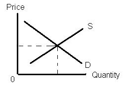
In summary, the demand curve shows the various quantities of a good that will be demanded (i.e., consumers are willing and able to buy) at various prices, while the supply curve shows the various quantities of a good that will be supplied (offered for sale by producers) at various prices. The point where the two intersect is the point where the quantity demanded equals the quantity supplied and this is the equilibrium or market price.


Equilibrium
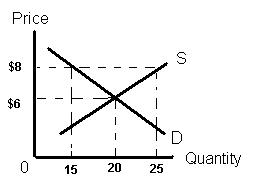
Question: "If the equilibrium price of a product were $6 and the actual price charged in the market were $8, you would expect?"

Answer: There will be a surplus or excess of product on the market since the quantity demanded by buyers will be less than the quantity supplied by sellers.



In the graph above, consumers only want to purchase 15 units of the good at $8, while sellers want to sell 25 units at that price. We have a surplus, or overstock, of 10 units (25 available for sale minus the 15 people are willing to buy). Since sellers are in business to get money, they will compete to get rid of their merchandise and the best way to lure a buyer from a neighboring store is to offer the identical product at a lower price. Each will begin lowering their prices until all of the product is sold. Sellers who were forced to sell below cost will drop out of the market (or at least drop that product line) so long as the price is below the $8 which brought them into the market. The market will then stabilize at $6 which is the price at which the quantity supplied equals the quantity demanded.

Question: "A decrease in equilibrium price and quantity in a market will be caused by?

Answer: Both the supply curve and demand curve show how quantity demanded or supplied changes as price changes with all other influencing factors being held constant. But you and I know that price is not the sole factor in determining what and how much we buy or how we choose to sell our labor or any other product we may have.

The other Determinants of Demand are:

1 Consumer Tastes

2 Income level of consumers

3 Size of population (or number of consumers in market)

4 Prices of other goods, specifically substitutes (goods that can be used in place of the good in question such as buying lower priced chicken in place of steak) and compliments (good used in conjunction with another good such as hamburger buns and hamburgers).

The other Determinants of Supply are:

1 Technology

2 Input prices (the cost of the inputs, such as labor, raw materials, etc., used in the production of the product in question).

In constructing the two graphs used above, we assumed that the other determinants of demand and supply, listed above, remained constant while only price changed. However, these other determinants can, and do, change. When they change the result is a shift in the supply or demand curve.

For instance, the question "A decrease in equilibrium price and quantity in a market would be caused by?" can be answered by a change in one of the determinants of demand such as:

1 Taste – if consumers become concerned about the increased risk of injury and death posed by compact cars they will change their tastes or preferences for compact cars and many will switch to larger vehicles which they perceive as being safer.

2 Income Levels – if wages in Tucson drop across the board, local consumers will have less money to spend and they will want less of a product at every price.

3 Size of Population – if the Air Force decides to consolidate the functions of DMAFB with those of another base in another state and move all of the personal from DMAFB to the other state the population of Tucson will drop and so will the number of homes/apartments needed to house the remaining population. In this case fewer homes/apartments will be demanded at every price.

4 Prices of Other Goods – if the price of chicken at KFC, Church's Chicken, etc. drops while the price of hamburgers at MacDonalds, Burger King, etc. remain the same, many people will switch from hamburgers and substitute the lower priced chicken causing the quantity demanded of hamburgers to be less at every price.

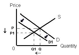
In each of the scenarios above, a change in one or more of the other determinants of demand results in the entire demand curve shifting to the left and intersecting the supply curve at a new point where both the price and quantity are lower.



As you can see in the graph above, the demand curve has shifted to the left, from D to D1, the equilibrium price has dropped from P to P1 and equilibrium quantity dropped from Q to Q1.

If the opposite happens in any of the above determinants of demand (i.e., tastes change in favor of the product, incomes go up, population increases or prices of other substitute goods increase - i.e., prices at chicken fast food restaurants increase but those at hamburger restaurants don't, making hamburgers relatively cheaper than chicken offerings) then the demand curve will shift to the right signifying that greater quantities are demanded at each price.

Further, if one or more of the determinants of supply increase, that curve will shift. An advance in technology that results in reducing the cost of production (such as a new process for making steel from iron ore that results in a reduction in the cost of producing steel – this will lower the cost of steel thereby reducing the cost of producing things like cars which use a lot of steel). This will cause the supply curve for cars to shift to the right showing a larger quantity supplied at every price. Similarly, a drop in the price of oil will result in lower fuel costs for airlines and this means that the cost of flying airplanes will be lower. This would shift the supply curve for air travel to the right showing increased quantity (i.e., more flights) at every price. BUT, if the price of oil increases, this will raise the cost of flying airplanes causing the supply curve for air travel to shift to the LEFT indicating fewer flights (lower quantity) at each price.

Gresham's Law

Most introductory economics texts make some reference to the so called “Gresham’s Law which is usually stated as “bad money drives out good money”. What this means is that when two types of money have the same face value within a region but are valued differently outside the region, the one with the higher value outside will be horded and the one with the lower value will be used for spending.

You are probably thinking “why a country would have two currencies and why the currencies have the same value within the country and a different value outside the country”. The economist Robert Mundell in an article entitled “Uses and Abuses of Gresham's Law in the History of Money” gives the example of gold or silver coins which have the same face value (i.e., all the quarters are worth twenty-five cents each) but, due to wear, the older coins have slightly less weight so that when they are melted down the older coins yield a lower amount of the precious metal. For day to day transactions, a thirty year old worn quarter is just as good as a brand new quarter when put in a vending machine or given to the cashier in the store. But, if you go abroad and try to sell the coins for their metal content you will receive less for the old coins than the new ones since the old ones have lost some of their gold or silver content due to wear. Therefore, people who have access to buyers of gold or silver will save the newer coins when they receive them and spend the older ones.

An example of this phenomenon occurred in the United States about forty years ago during the 1960s when the price of silver began to rise. Up until that time dimes, quarters and half dollars were almost 100% silver (an alloy was added to increase hardness and decrease wear and this resulted in their not being pure silver). At this point the U.S. Treasury had the mint reduce the silver content by manufacturing “sandwich” type dimes, quarters and half dollars using a copper alloy center with a layer of silver on the top and bottom. Except for the copper colored center when observed sideways, the new coins looked and felt the same as their older silver counterparts. But the value of the silver and copper in the new coins was less than the face value of the coin (i.e., if you melt down a quarter the value of the resulting metal is less than twenty five cents) while the value of the silver in the old coins was worth more than the face value of the coin. The old, pre-1960s dimes, quarters and half dollars and the new, post 1960s dimes, quarters and half dollars are still legal tender and can be used interchangeably for purchases. BUT, all of the old silver coins have disappeared into coin collections or have been melted and sold for more than their face value. If you should be fortunate enough to encounter one of these old coins, which, look like the present ones, keep it as it is worth considerably more than the ten, twenty five or fifty cents exchange value in a store.

And, who was this Gresham fellow who postulated this law? Sir Thomas Gresham was a successful businessman and financial adviser to Queen Elizabeth I (1533 – 1603) who observed the phenomenon, like many before him, that when two currencies have the same face value at home but are valued differently abroad, the one with the higher value abroad will be horded and the one with the lower value used in exchange locally. While this had been observed and written about for twenty centuries before Gresham made the observation, it was Gresham whom the British economist H. D. Macleod referred when Macleod described the phenomenon in a publication in 1858 and named it “Gresham’s Law”.